How Healthy is the US Labor Market?

The plunge in labor force participation since the great recession in 2008 has led many to rightly question how well the unemployment rate -- the percent of the labor force that has looked for work in the last 4 weeks -- measures the true level of "slack" in the labor market.

Much (most) of the decline in labor force participation can be explained by the retirement of baby boomers, the oldest of which turned 65 in 2010, and by people between the ages of 16 and 24 choosing to focus on education instead of working.

The decline in labor force participation among young people is something that was occurring before the great recession. Even though it the recession seems to have sped up the decline, I'm pretty certain that most of the people between 16 and 24 who left the labor force in 2008 and 2009 or simply haven't joined since then (I'm in that group) wouldn't rejoin even if there was no slack in the labor market.

While the labor force participation rate for Americans 55 and older didn't actually decline in the great recession, it stopped a decades-long trend upward and has flattened out since then.

The fact that the participation rate for older Americans has settled at a lower level than participation for the general public, and that the share of the civilian noninstitutional population (basically everyone above the age of 16 who isn't deployed in the military or in prison) that is older than 55 years is increasing, has put significant downward pressure on the total labor force participation rate.

That being said, it's hard to be certain whether or not the recession has had lasting cyclical impacts on labor force participation, which warrants using statistics other than the unemployment rate to gauge the strength of the labor market.

One such popular measure is the broadest measure of underemployment put out by the Bureau of Labor Statistics (BLS) -- total unemployed, plus all marginally attached workers plus total employed part time for economic reasons -- or the U-6 unemployment rate.

I don't really like this as a measure of labor market strength though, because it doesn't count people who retired earlier than they wanted to as a result of the recession, people are only counted as "marginally attached" if they have searched for work in the last 12 months, and part time workers aren't really unemployed (there is an alternative measure that excludes involuntary part time workers but it still has the problems I mentioned above).

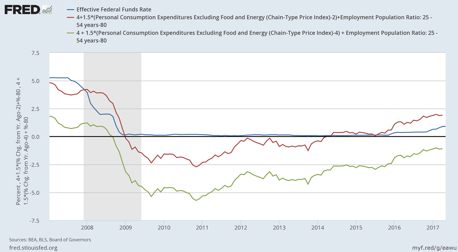
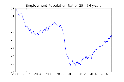
Some people like to look at the employment rate for the so called "prime age" population who are between the ages of 25 and 54 (I don't know why the cutoff is 54, going up to 65 makes way more sense to me) in order to weed out the effects of aging and lower youth participation on the labor market.

This is a relatively good solution for the years after 1990, and it does show that the labor market is considerably weaker than the unemployment suggests (although not so weak that we need to "prime the pump"), but it has trouble before 1990 because women were still joining the labor force en masse for most of the latter half of the 20th century.

Basically every statistic that you can easily get from BLS data has a problem like this, so it's really hard to get a good measure of how healthy the labor market is, but there is a solution. The Congressional Budget Office (CBO) looks at the demographic composition of the working age population and comes up with what it thinks the labor force participation rate would be at full employment. It calls this measure the "potential labor force", which tries to estimate the movement in labor force participation caused by gender and aging and can then be used to estimate the cyclical component of labor force participation.

It is then possible to find the "adjusted" unemployment rate with the CBO's estimate of the potential labor force. The above chart shows the actual unemployment rate reported by the BLS as well as my calculation of the adjusted unemployment rate using the potential labor force from the CBO's 2007 and 2017 data for "Potential GDP and Underlying Inputs" (all CBO data is available here). The dashed grey line is the natural rate of unemployment -- that is the unemployment rate that is consistent with full employment -- according to the CBO.

Since I was only able to find annual "potential labor force" figures, the estimates only extend to 2016, but both the 2007 and 2017 figures are broadly consistent with the prime age employment rate: the unemployment rate overstates the health of the labor market by between 1 and 2 percent (depending if you use the 2007 or 2017 value for the potential labor force). This is similar to where we were in 2003 or 1994, so while there's no real cause to worry about joblessness right now the recovery isn't completely over yet either. As a side note, tax cuts are even more of a stupid idea now than they were in 2003, but that issue deserves a whole post of its own.

Is Raising the Inflation Target Possible (Right Now)?

Ever since a group of 22 economists wrote an open letter to the Federal Reserve advocating for an increase in the inflation target, economics blogs have been abuzz with discussion about the merits of a targeting an inflation rate greater than 2%.

While I don't have much to say about the value of changing the inflation target (I pretty much agree with the authors of the letter), I do think there are several practical issues that the Fed would have to deal with if it did want to start targeting e.g. 4% PCE inflation.

As I see it there are currently two obstacles that make it practically hard for the Fed to increase its inflation target: 1) the Fed doesn't have enough credibility, and would squander what little it has if it tried, to raise inflation and 2) interest rates are so low that providing the necessary stimulus to get inflation to 4% is basically impossible in the short to medium term.

The Fed adopted a 2% inflation target in 2012 after unofficially targeting 2% inflation for years up until that point, but ironically core PCE inflation has not been 2% since March of 2012 (the headline rate was briefly 2.15% this February).

This consistent undershoot of the inflation has begun to take its toll on the Fed's credibility, with both expected inflation measured by the University of Michigan survey of Consumers and spread between normal treasury securities and inflation protected ones falling below normal levels after 2014.

Since the Fed can't even meet its own low inflation target, what makes anyone think it can meet a higher one? Before we even think about raising the inflation target, we should make sure the Fed is actually capable and willing to let inflation reach 2%. If it that doesn't happen, I'm skeptical that markets and consumers (who are probably too backward looking to expect inflation until they've been experiencing it for a while anyway) will take an increased inflation target seriously.

Beyond just announcing that it is now targeting a higher inflation rate, say 4%, the Fed would have to take concrete action to raise inflation to its new target. This would involve lowering interest rates considerably, because inflation would now be about 2.4% below target instead of just 0.4%. A useful way of thinking about this is comparing a Taylor Rule with a 2% inflation target and one with a 4% inflation target.

Here the blue line is the actual Federal Funds rate, while the red line is what a Taylor Rule -- with a coefficient of 1.5 on inflation and 1 on the "output gap" (in this case defined as the difference between the prime age employment rate and its "full employment" level of 80%) -- would suggest the interest rate be with a 2% inflation target. The green line shows what interest rate we should expect the Fed to set given a four percent inflation target. Basically, in order to commit to raising inflation to 4%, the Fed would have to either find a way to make interest rates significantly negative or otherwise go back to the zero lower bound for the foreseeable future.

I know that even the people who signed the letter weren't suggesting an immediate switch to a higher inflation target, but to the extent that they want the change to happen in the next few years, during which the economic climate will probably remain about the same, it's unclear as to whether or not a quick increase in inflation is actually that possible.

Microfoundations, the Euler Equation, and the Phillips Curve

Late last night (early this morning for everyone in America?) I had a conversation on Twitter with Noah Smith that got a lot of attention, and later turned into a discussion with with Jonathan Hyde about the New Keynesian Phillips Curve.

The actual thread is pretty long and confusing, so I'll just summarize it here. First in a sort of tongue-in-cheek way I asked Noah why economists model agents rationally when they are evidently not rational. He and I then went back and forth about empirical evidence, and I said "Well the Euler equation at least is patently wrong, and the NKPC [New Keynesian Phillips Curve] has trouble explaining inflation since 2008," which led to everyone's favorite tweet of the night (after my joke about how the models in Physics actually work):

Incidentally if both Euler equation and NKPC are wrong, then workhorse NK model is basically refuted

— John Handleyハンドリージョン (@jwhandley17) June 14, 2017

 This is where Jonathan came to the defense of the NKPC:

... demonstrated (as far as I can tell) that more plausible models of price stickiness (e.g. menu costs) make any significant difference.

— Jonathan Hyde (@Britonomist) June 15, 2017

 While his comment is not wrong, I think it points to one of the main problems with macro: insistence on modelling the underlying factors behind observed phenomena like the Phillips Curve, aka obsession with microfoundations.

The expectations augmented Phillips Curve has been around since the late 1960's, but microfoundations meant that economists spent years trying to figure out why rational optimizing firms would not adjust their prices instantly -- for a while the debate was between Taylor contracts and menu costs as a source of nominal rigidity -- but eventually settled with the mathematically tractable hand wave that is Calvo pricing.

The Calvo model basically says that firms face a constant an exogenous probability that they will not be able to change prices in the next period, so they might set their price too high or too low this period so that they won't be stuck with an extremely suboptimal price next period. This obviously doesn't classify as a "microfoundation" in that it doesn't appeal to a friction that actually exists in the real world.

In principle, microfoundations might seem like a good idea since they help deal with the Lucas Critique that relationships that appear in the aggregate data -- like the relation between inflation and unemployment -- might disappear when they are exploited. The problem comes when you realize that models with perfectly rational utility/profit maximizing agents don't work empirically. When that fact becomes clear, there are two options: add a whole bunch of implausible assumptions about agents (like Calvo pricing or habit formation) to make the model fit the data or just go back to modelling things ad hoc.

Economics has mostly gone with the first approach in the last 30 years, adding tons of parameters (e.g., the fraction of firms that cannot change their prices in a given period, the degree of habit formation, the elasticity of demand for individual monopolistically competitive firms, etc.) to a model just so they can come up with models that behave a lot like the old ad hoc models.

I don't think that economic incentives shouldn't be considered when making modelling decisions, but frequently models with completely rational agents and utility maximization produce results that go too far. A key example of this is consumption. In my last post I showed that consumption is pretty much entirely explained by income and wealth, which is a prediction of the Permanent Income Hypothesis (PIH). Essentially, agents try to "smooth" consumption in the face of shocks to income, so they consume out of their wealth when their income falls and save when income is high. A slight amount of consumption smoothing also occurs when people become unemployed. The consumption Euler equation also predicts consumption smoothing, but to an absurd degree. Whereas Jason Smith and I found that consumption is highly receptive to changes in income, the Euler equation predicts complete consumption smoothing.

A more ad hoc consideration of economic incentives and the economic data would lead to a highly qualified version of the PIH that does a much better job empirically than a strict utility maximizing approach. The same thing goes for the Phillips Curve, where assuming rational expectations makes the relationship statistically insignificant (see the t statistic on u_gap, the gap between the unemployment rate and the Congressional Budget Office's estimate of the natural rate of unemployment, in the table below):

Ultimately, in my opinion, the empirical failures of microfounded models show that trying to rigorously model the underlying causes of relationships we see in the aggregate data is a waste of time. Business cycle theory in particular should be more empirically oriented and less focused on logical consistency.

Update: here's a link to the code where I compare the New Keynesian Phillips Curve and a backwards looking Phillips Curve to the data.

Modelling Consumption

I was running over things to write about over the next few weeks, and I decided to just casually see how much income and wealth explain consumption. I didn't expect to see anything spectacular, but I pulled the quarterly personal consumption expenditures series as well as disposable personal income and household and nonprofit net worth and ran a regression. The IPython notebook is here.

At first I ran the regression on all the data from 1952 on, and the result actually shocked me -- the first time I think I can say that while referring to statistics -- the R squared value was literally 1. I was too surprised to look at the p values or t-statistics for each variable, but I decided to only look at data after 1990 to see if that changed anything.

Here's the output for the regression on data after 1990:

I still suspect that I did something wrong here, but the fit is, in a word, impressive.

I also plotted the prediction given the coefficients from the regression against the actual data:

For good measure, these are the series IDs from FRED I used: Personal Consumption Expenditures: PCEC, Disposable Personal Income: DPI, Households and Nonprofit Organizations; Net Worth, Level: TNWBSHNO.

Update: I removed wealth from the regression, and the fit is still extremely high. I guess now the question is, if disposable income is such a good predictor of consumption, why does the Old Keynesian consumption function get routinely bashed for being inaccurate? Yes, I know the difference between average and marginal propensity to consume is important, but why insist on the consumption Euler equation given it's almost comical level of inaccuracy while ignoring the startlingly accurate Keynesian consumption function?

The results of the regression without household wealth:

Update 2: At Jason Smith's suggestion, I looked at the correlation with first differences (really 4 quarter growth rates) and found that the R squared went down to more normal levels, but that adding wealth does actually improve the fit considerably. The importance of wealth here is a partial win for the Permanent Income Hypothesis but ultimately still a loss for the consumption Euler equation. Here are charts for the new regression:

Monetarism and the Neo-Wicksellian Framework

I know I'm about a year late to the party, but recently I have been listening to David Beckworth's Macro Musings podcast. Two interviews that particularly caught my attention were the one with Nick Rowe and the one with Brad Delong. In the ten months since Brad and Nick were on the podcast the world has been too preoccupied with Donald Trump's antics and, more recently, the snap general election in the UK to do much discussion of economics, but now I want to talk a little bit about the relationship between monetarism and new Keynesianism.

Both Brad and Nick argue when talking to David that new Keynesians are really all monetarists, or, more specifically, that in the 1990's everyone agreed that economic fluctuations were caused by disruptions in the demand and supply for money and that the big question was what rule should replace Milton Friedman's k% rule for monetary policy. According to Nick, the absence of money in new Keynesian models is really just implicit because if the model had no money (i.e. if it were a barter economy) agents would just "barter their way back to full employment."

I think the idea that recessions are just excess demand for money is interesting, especially since it applies even in the very Keynesian context of IS-LM. With the LM curve relating real money demand to output and the interest rate, it is clear that shifts in the IS curve are the same thing as higher demand for money at a given interest rate. If we write the LM curve as M/P = L(Y,r) = aY - br and the IS curve as Y = c - dr, then we can figure out what happens if a recession hits -- in this case that means c falls. In a normal IS-LM diagram, the IS curve would shift left, and both r and Y would fall, but if you look at it slightly differently by holding Y constant given the fall in c, you can see that a shift in the IS curve just changes the level of r for a given Y. Substituting this back into the LM curve shows that money demand for a given level of Y has increased: M/P = aY - br = aY - b/d(c+Y) = (a - b/d)Y -b/dc.

That might be really confusing, and I apologize for not being able to explain things as succinctly as Nick can, but basically I'm saying that recessions (drops in aggregate demand) are just increases in the demand for money (given the level of real GDP) that are not met with increases in the supply of money. Since the quantity of money demanded must equal the quantity supplied, output falls to reduce money demand to the appropriate level. That's why if c falls by, for example, 10 in the model above, then the real money supply must increase by b/d*10 for output to remain constant.

Bringing expectations into the money demand function makes things a little more interesting. Let's say money demand increases when inflation expectations are low because, per the fisher equation, low inflation expectations mean low nominal interest rates and low interest rates cause less incentive for people to hold interest bearing assets in place of money. In this case, if something causes inflation expectations to fall precipitously, money demand will increase and, absent central bank action to increase the money supply, a recession will occur. If, as is true in most cases, central banks have control over inflation expectations in the medium to long term, they effectively have the power to shift around the demand for money. Thus, monetary policy can take two forms: open market operations and expectations management.

This is where Neo-Wicksellian comes in. I've written a little bit about this before, but monetarists usually prefer the money demand/supply description of monetary policy because they see interest rates as a bad indicator of economic conditions (never mind that wild swings in money demand also make most measures of the money supply bad indicators of economic conditions). I, however, think that the monetary explanation of business cycles and the Neo-Wicksellian description are very similar, but that using interest rates has a couple of distinct advantages.

In its simplest form, the Neo-Wicksellian framework just says that if the central bank sets a nominal interest rate above the natural interest rate, there will be a recession and vice versa. Thus, with a relatively constant natural interest rate, high interest rates lower aggregate demand while low interest rates raise aggregate demand. The problem is that the natural rate of interest -- which you could consider as the level of r that keeps Y constant in the IS curve above -- fluctuates around a lot, which makes interest rates look procyclical.

Another important thing to notice is that central banks can influence the natural rate by changing inflation expectations, which is basically the same as how they change money demand. In way, the Neo-Wicksellian framework in which recessions are equivalent to interest rates above the natural rate of interest and the "monetarist" view in which recessions are excess demand for money are basically the same thing, just with the focus on different variables.

The Neo-Wicksellian view does have one advantage in my opinion though: it more accurately shows constraints on monetary policy. In the monetarist view, the solution to a shortfall in aggregate demand is always more money, but the Neo-Wicksellian view shows that there are constraints to monetary policy, at least in the present. If the natural interest rate falls below zero, the central bank no longer has the ability to just cut interest rates/just increase the money supply to ward of a recession. At this point, the only way a central bank can end the shortfall in aggregate demand is to increase expected inflation so that the natural interest rate is no longer negative. This is why increasing the monetary base from about $800 billion to about $1.7 trillion didn't stop GDP from collapsing in 2008.

Given that Neo-Wicksellian and monetarist frameworks both work as ways of looking at the same IS-LM model, I don't know how valid it is to say that everyone became a monetarist or that everyone became a "new Keynesian" in the 1980's and 1990's. It seems like there really isn't that much difference between either group in the first place. At least over the last few years, the real split in economics seems to be between people like John Cochrane who are skeptical of sticky prices and that fiscal policy can raise aggregate demand at all and everyone else.